The Chi-square test of independence (also called the Chi-squared test) is a standard measure of association between two categorical variables. It determines whether there is a significant relationship between the variables. If the two categorical variables are independent of one another, knowing the value of one provides no information about the value of the other variable. If one depends on the other, it can be worthwhile to examine their relationship.
The crosstab takes care of doing the Chi-square test for you, but it can be useful to understand how the system derives the values in question.
We're going to use gender as our first categorical value and favorite colors as our second.
What is your favorite color? | ||||||||
Gender | Yellow | Green | Blue | Red | Orange | Black | Purple | Row Total |
Female | 137 | 320 | 754 | 369 | 74 | 159 | 449 | 2262 |
Male | 59 | 343 | 1188 | 454 | 120 | 155 | 112 | 2431 |
Column Total | 196 | 663 | 1942 | 823 | 194 | 314 | 561 | 4693 |
Now we compute the variable counts we would expect if the variables are independent. The row and column totals are used to calculate the expected counts for each Gender/Color combination. So we multiply the row total by the column total, then divide that by the grand total.
For the Male/Orange combination, that's 2431 * 194, which is 471614, divided by 4693. Our expected value (rounded to the nearest whole number) is 100. I've put the expected value for each cell in parentheses and used red text to differentiate it.
| What is your favorite color? | ||||||||
| Gender | Yellow | Green | Blue | Red | Orange | Black | Purple | Row Total |
| Female | 137 (94) | 320 (320) | 754 (936) | 369 (397) | 74 (94) | 159 (151) | 449 (270) | 2262 |
| Male | 59 (102) | 343 (343) | 1188 (1006) | 454 (426) | 120 (100) | 155 (163) | 112 (291) | 2431 |
| Column Total | 196 | 663 | 1942 | 823 | 194 | 314 | 561 | 4693 |
Now we will calculate the difference between the actual and expected values for every combination, square that difference, and divide the result by the expected value for that cell. Adding all of those values gives us the test statistic. Using our Male/Orange cell as an example, the actual value is 120. The expected value is 100. The difference is 20, and squaring 20 gives us 400. Dividing 400 by 100 gives us 4. I've placed that in curly brackets and used green text to differentiate it.
| What is your favorite color? | ||||||||
| Gender | Yellow | Green | Blue | Red | Orange | Black | Purple | Row Total |
| Female | 137 (94){19.67} | 320 (320) {0} | 754 (936) {35.39} | 369 (397) {1.97} | 74 (94) {4.26} | 159 (151) {0.42} | 449 (270) {118.67} | 2262 |
| Male | 59 (102){18.13} | 343 (343) {0} | 1188 (1006) {32.93} | 454 (426) {1.84} | 120 (100){4} | 155 (163) {0.39} | 112 (291) {110.11} | 2431 |
| Column Total | 196 | 663 | 1942 | 823 | 194 | 314 | 561 | 4693 |
To get our test statistic, we add all the values in green to get 347.78. That's our Χ2 statistic.
Next, we need to calculate our degrees of freedom (df), which depends on how many rows and columns we have. The formula is df = (r - 1) * (c - 1). We have 2 rows and 7 columns, so df = 6.
We need our significance level, α. CivicScience uses a significance level of 0.05 for all crosstabs.
Now we use a published Chi-square distribution table to look up the value for those values. It's 12.592.
When we compare the value of our test statistic (347.78) to the Chi-square value of 12.592. Because 347.78 > 12.592, we reject the hypothesis that gender and favorite colors are independent. We can conclude that the variables have some kind of relationship, though we can't say what kind.
Here are the same variables shown in a crosstab. The percentage of difference from the expected value is shown if it is significant. The variables show a high strength of association, as stated in the summary line at the bottom.
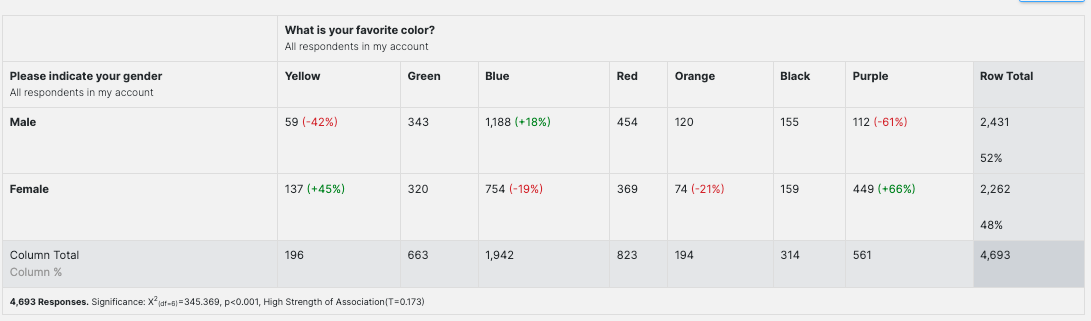
In the summary line, you'll see the number of responses, the significance expressed by the Χ2 value, the df (degrees of freedom) value, the p-value, and the strength of association, which uses the T coefficient.
Χ2 is the Chi-squared statistic. This one is slightly different from what we calculated above due to rounding differences.
We also calculated our degrees of freedom (df) above.
The p-value corresponds to the Chi-squared statistic and represents the probability that there is no relationship between how respondents have answered each question. The lower the p-value, the more confident we can be that such a relationship exists. Results that are shown to be statistically significant have been adjusted according to the Benjamini-Hochberg false discovery rate procedure.
The T coefficient is Tschuprow's (sometimes spelled Chuprov's) T. Tschuprow's T is a measure of the strength of the relationship between how the respondents answered each question. Its value ranges from 0 to 1. The higher the value for Tschuprow's T, the stronger the relationship between how the respondents answered each question.